Autonomous Robotics at Beaver Works Summer Institute
The program
The Beaver Works Summer Institute (BWSI) began as an idea by Dr. Robert "Bob" Shin of MIT Lincoln Labs to create a summer program for programmers, an area that was previously undeveloped. His goal was to create a program where high school students from around the United States could work together with top researchers and professionals in the field of robotics to develop autonomous robotics systems. In order to find students for the pilot year of BWSI, Dr. Shin contacted the National Consortium of Secondary STEM Schools (NCSSS) and was able to find students from many of the member schools. Students came from 11 states: Mississippi, Illinois, Arkansas, California, New York, Maine, North Carolina, South Carolina, Virginia, New Jersey, and Massachusetts.
The program lasted for 4 weeks. The students worked each weekday from 9:00am to 5:00pm. During the weekdays, the students listened to lectures and seminars and worked on labs to enforce the material and accomplish weekly goals. On Tuesdays and Thursdays, the students would also attend a lesson on communication with Dr. Jane Connor. Each week, the students were given a section of robotics to learn and a challenge.
Week 1 focused on the basics of the basics of the Robot Operating System (ROS), Linux (Ubuntu), and Python. The challenge for the week was to make the robot follow the wall using the Lidar.
Week 2 focused on image processing and recognition (manipulating and matching images). The challenge for the week was to visual servo (approach using visual input for steering) to a target on the wall and decide which direction to turn based on which color, red or green, is present.
Week 3 was intended to be focused on localization and mapping, however, several technical issues led to a focus on the technical challenges instead. These challenges included exploring and detecting colored blobs and completing a correct turn at a colored piece of paper.
Week 4 was focused on final preparation for the Grand Prix, the final challenge. The Grand Prix was to be a race around a miniature Grand Prix circuit, complete with shortcuts and sharp turns. During this week, the Grand Prix was hosted and tech challenges were completed.
The Car
Chassis
The cars used ion this project were built off of the Traxxas Rally 74076 chassis. This chassis was used because of the Ackermann drive (front wheels used for turning) and high speed capabilities, up to 40mph.
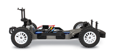
Basic car chassis [1]
Processor
The processor used on the car was a Nvidia Jetson TX1. This is an embedded system that uses a GPU to complete the processing. This means that the board has hundreds of cores that complete processes rather than two or four cores. This makes visual computing very fast.
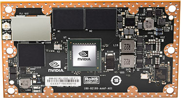
Nvidia Jetson TX1 Module [2]
Sensors
Numerous sensors were used to allow the car to be able to sense its environment.
Active Stereo Camera
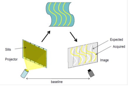
The active stereo camera uses a projector and camera to produce and read the disturbances in structured light. This allows the camera to give distances in a point cloud. A point cloud is a data structure that holds points at different angles with distances associated. [3]
[3]
Passive Stereo Camera
Passive stereo cameras sense distance using the discrepancies in the images that two cameras capture. This is accomplished by matching objects on two images and finding the offset between them. depth = f (b / d) where depth is the distance to the object, f is the focal length of the camera, b is the distance between the cameras (baseline), and d is the disparity in pixels. [3]
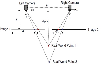
Process of finding distance using passive cameras [3]
Inertial Measurement Unit (IMU)
The IMU is used to measure linear acceleration and angular acceleration. It accomplishes this through the use of capacitors and springs on nanoscale that shift when accelerating.
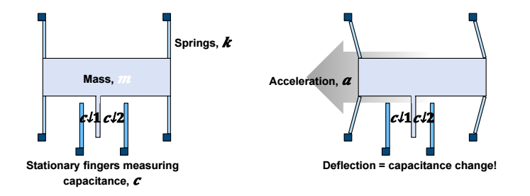
Deflection changing capacitance shown [1]
2D Lidar
The Lidar system uses light to measure distances from the robot. This is accomplished by shooting a laser in an arbitrary direction and timing how long the light takes to return to the robot.
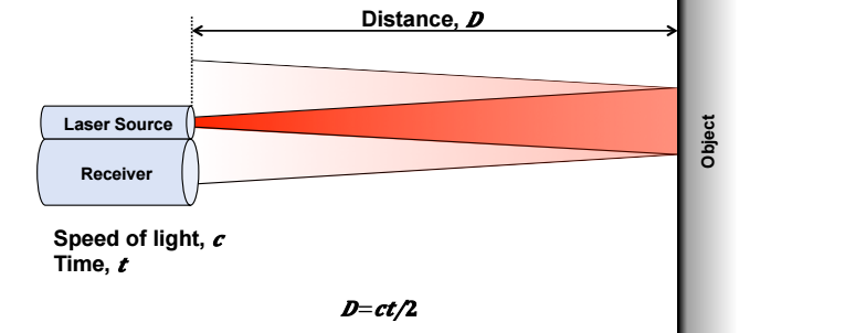
Mechanism used to measure the distance [1]
Full Car
All of the sensors were placed on the robot as shown below. The passive stereo camera was placed where the active stereo camera is shown and the active stereo camera was removed. A wireless router was placed on top of the robot to allow the robot to have a lower disconnection rate.
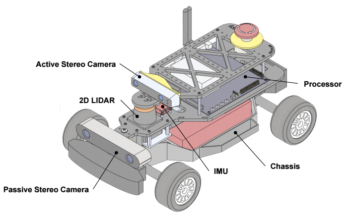
Car with all sensors [1]
Week 1
Goals
There were several goals for week 1. The first goal was to level the playing field for all students by reteaching everything from the summer work. The next goal was to learn how to use the LIDAR to interpret the environment and follow a wall.
Lectures
The first day of the program was intended to explain the basics of the cars we were using. The Jetson TX1 is the processor we used. This is a special processor with hundreds of cores that allow for fast parallel processing. ROS is based upon the idea of parallel processing and, as such, works well with the Jetson. We decided to use a special distribution of Ubuntu for the Jetson. ROS runs on Linux and Ubuntu is a very easy version to use. On top of the cars are wireless routers that allow the robot and our computers to connect to each other and the internet. An electronic speed controller (VESC) is used to control the driving speed and steering angle of the robot. A passive stereo camera is used to sense depth and input images. A LIDAR is used to perceive distances in a horizontal plane in a 270° angle.
The next day we learned about the basics of Linux, Python, ROS, and robotics. We learned the basics of the Linux shell, Python syntax and tricks, ROS topics and nodes, and robotic architecture.
Kyle Edelberg taught on control systems and how he used them at the MIT Jet Propulsion Lab in California (JPL). The basic control systems are Open and closed loop control. In open loop control systems, there is feedback that determines the next adjustment. In closed loop control systems, there is no feedback to help with control and thus they are more unstable. He lectured on the use of proportional, differential, and integral controllers (PID controllers). PID controllers work by first having a way of defining an error. This error is passed into the PID controller and a steering command is output. The controller has three parts. Proportional is the part that points the car toward the way to reduce the error. Derivative uses the change in the error to slow the acceleration toward the point of no error. This effectively prevents destructive oscillatory motion and overshooting. The integral portion prevent steady state error. These are errors that persist and the robot cannot correct for. They are removed by keeping a tally of the errors over a frame of time.
Labs
We connected to the cars and learned how to publish topics. Topics are channels of communication between nodes that allow for easy transfer of data. Nodes are individual parts of a robot such as a sensor, motor, controller, or output device.
We ran nodes to demonstrate communication between ROS nodes. We also learned how to simulate a physical environment using the gazebo simulator.
We used rviz to see the output from sensors on the robot and rosbagged all topics in order to understand what happens when the robot runs. Rosbag is a command in ROS that saves data published to topics in real time.
The team implemented a Bang-Bang(BB) controller and a PD (Proportional and Differential) controller. BB controllers are essentially binary controllers. If the car is too close, the BB will push the car full in the opposite direction and vice-versa if the car is too far. The controller has two states: full left and full right. PID controllers adjust to the error in a controlled manner that prevents large switches and inefficiencies.
The algorithm for the PD controller was implemented in the following way:
Conclusion
The team implemented a wall follower that could switch which wall was being followed using a gamepad. This program used the shortest distance from the robot to the wall in a range of the laser scan to find the error. This error was then fed in to the PD controller which determined the steering angle for the car to drive. The team placed 4th in the first round with a time of 8.645s [4]. In the drag races, we progressed past the first round to be defeated by the “Fastest Loser” in the second round. The team dynamic was very healthy and enjoyable. We all learned how to deal with others' opinions and criticisms. We chose each other when were allowed to choose teams for the final weeks.
Week 2
Goals
The goals for week 2 were to be able to use blob detection, visual servo toward a blob, and recognize different colored blobs. Blobs are colored swatches. Contour has a similar meaning; a contour is an area of a similar color of an area that fits inside a certain criterion. We used pieces of paper for the blobs. Visual servoing is following a blob toward a target.
Lectures
Monday focused on color spaces and segmentation. Color spaces are the various was of storing colors for pixels. The normal way that most people think about color and most computers use is called the RGB color space. This color space stores values that relate to the intensities of each form of light in a pixel. rgb(255,128,0) means that red has full intensity, green is at half intensity and blue is off. This would make a color like this. The BGR color space works in the same way, but reverses the order of each color. bgr(255,128,0) means that blue has full intensity, green is at half intensity and red is off. This would make a color like this. These color spaces are difficult to use in visual processing because lighter and darker conditions cause wide variances that cannot be easily accounted for, enter HSV. HSV stands for hue, value saturation. Hue is the absolute color from 0 to 360. In the code however, the wheel was condensed to 0 to 180. Value is how dark or light the color is (black to vibrant). Saturation is how washed out the color is. This goes from white to vivid. hsv(180,170,170) has a hue of blue-green, a medium-high value that makes it darker and a medium-high value that makes it washed out a bit. The color looks like this. The HSV color space is very useful in image processing as it is easy to designate what approximate hue you want. Hue specifies the color, saturation is used to account for whitewash, and value is used to adjust for brightness.
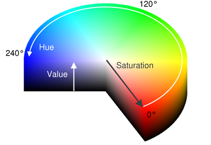
HSV Color Space Graph [5]
Segmentation is using as binary mask to select parts of an image. A mask is an boolean, two-dimensional array that represents an image. If a certain pixel matches a pattern, the bit at that index in the array becomes true. Masks are used to show areas of an image where a certain criterion is true. These criteria are ranges of HSV values. An example would be: mask = cv2.inRange(image_in_hsv, numpy.array([0, 100, 200]), numpy.array([15, 255, 255])). This goes through the image and finds any pixel with hues between 0 and 15, saturation between 100 and 255, and value between 200 and 255. In our lab this found a piece of paper on the wall.
Tuesday focused on programming the robot to use visual input. The lectures focused on using the passive stereo (ZED) camera with ROS, detecting blobs, and visual servoing. The passive camera published to the following topics in the camera namespace: rgb/image_rect_color, depth/image_rect_color, rgb_camera_info. The programs subscribed to the /camera/rgb/image_rect_color topic which published RGB images from the camera. Blob detection is using openCV to group clusters of true indexes in masks. This allows programmers to determine the size, shape, and location of detected objects. The locations of these contours are used for navigation called visual servoing. Visual servoing is the use of an inputted image to determine the appropriate action.
Labs
The goals of the first lab was to subscribe to an image stream (the /camera/rgb/image_rect_color topic) and edit images as they come in from the zed camera. The three manipulations that were required were adding a shape overlaying the image, flipping the image about an axis, and adding a rosy appearance by increasing the red value of each pixel [6]. My team was unable to complete these three objective due to problems with the passive stereo camera. The next lab involved creating a custom message, publishing and subscribing to it, and detecting blobs. My team was able to complete this challenge. We accomplished this by writing the following script: On Wednesday, the weekly challenge was given, the goal was to drive toward a colored piece of paper and, depending on the color (red or green), turn right or left. This challenge was especially hard for most groups and only 2 of 9 teams were able to complete it. My team was not one of the two. The team was able to visual servo toward the wall and was also able to follow the wall on either side, however, we were not able to connect the two parts of the program to allow simple flow from visual servo to wall following.
Conclusion
My team was able to complete the main objectives of the labs but we were unable to complete the weekly challenge. The failure to complete the final challenge was due to a lack of communication within the group. Though the team had a large amount of knowledge, we were unable to connect and work together well.
Week 3
Goals
The objectives of week 3 were to learn localization and mapping. Due to technical issues, the goals shifted to learning about exploration and different ways of navigating free space. The final goals were to learn potential field navigation, free space navigation, and gradient fields and to detect numerous colored blobs as the robot explored the environment.
Lectures
The lectures this week did not necessarily correlate to the material of the labs. Monday focused on basics of simultaneous location and mapping (SLAM). This means moving and drawing a map as the robot moves. The rest of the week focused on exploratory algorithms (most days were lab time).
Labs
Monday's lab was to create a map using the SLAM approach. SLAM uses Lidar and odometry to assume the robot's position and draw a map. As the robot moves through an environment, it read the LIDAR and adds the reading to the map, the robot then adjusts its current assumed position to align with the more detailed map. It continues through many iterations of this to build a highly detailed map of the surroundings. Most robots were able to build a very low quality map which was due to very imprecise odometry.
Tuesday's goal was to be able to navigate a racetrack that was full of obstacles to avoid. Most teams were able to accomplish this through various methods. My team used the potential field method. This method used each point in the LIDAR scan as a point charge and placed a large point charge behind the robot. All charges were positive and pushed the robot away from obstacles and forward. The equations that describe the direction and speed are \(speed=\sum{sin(1/d^2)}+pushingCharge\) and \(direction=\sum{cos(1/d^2)}\). A major issue to this approach is the chance of reaching a local minimum where there is a low enough potential field vector that the car stops. To rectify this, the team added a stuck function that checked if the car was stuck and, if so, backed up for a second before resuming.
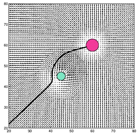
[7]
Other approaches the group tried were gradient fields and largest free space. Gradient fields assigned slopes at each point in the area around the robot, this led the robot to "slide" toward the goal and away from obstacles. My team decided against this approach due to added complexity and similar function to potential fields. Largest free space was also implemented and rejected due to lack of robustness. This approach found the largest free space each iteration and set the steering in that direction. This approach was faster and simpler but could not recover from crashes or slowdown on sharp turns.
The final challenge of the week was to explore and identify colored blobs in the track. My team was able to correctly identify most blobs and came in second among the other teams.
Conclusion
This week was a great success. Most teams were able to discover blobs as they traveled around and report them to a custom topic.
Week 4
Before Race Day
The final lecture was given by Dr. Sertac Karaman, Lead Instructor. This Lecture focused on the importance of autonomous vehicles and how the knowledge from the camp can be applied outside of the camp. The rest of the week was dedicated to preparation for the races and technical challenges. The code freeze for the tech challenges was at 11:15 on Tuesday and for the grand prix was at 5:00 on Friday.
The team worked to hack together the different programs we had written throughout the past four weeks to create a single program that could be used to compete. We decided on using potential fields for both the time trial and grand prix in order to avoid cars and quickly navigate. Although the challenge specification was to determine whether or not to go down the shortcut based on the color of the blob, we decided to always go right to be safe by adding an extra point charge to the left of the car to push it to the right.
Technical Challenges
The first tech challenge was to navigate and detect blobs. The team excelled on this part and detected most of the blobs in the area with few misidentifications. The second challenge was to detect the color at the entrance of the shortcut. The team was unable to program a correct solution to this challenge and decided to sit out instead. During the navigate and detect challenge, the servo on out robot began to overheat and then was struck by another team's robot causing it to die. We then had to change robots for the final grand prix.
Exploration Test
Time Trial
For the time trial, we decided to use our grand prix code which used a potential field for navigation. This last minute change allowed use to very quickly navigate the turn and never go down the shortcut when we weren’t supposed to. We earned 3rd place in the time trials securing us a place on the front row for the grand prix.
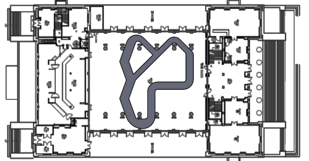
Final Grand Prix Circuit Map
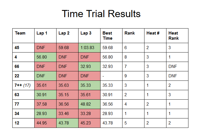
Results of the Time Trials [8]
Heats
The first heat was made up by the first, second, and third place teams. We competed in this heat and placed second putting us in the middle of the front row for the grand prix, the ideal position for our potential field navigator.
Grand Prix
This event was just for fun. All 9 racecars were placed on the track simultaneously and drove around until their batteries ran out. Many robots became turned around and blocked each other but overall, the robots all ran very well.
Conclusion
Technical
Over the course of this program, I developed a good understanding of autonomous systems and how robots are programmed. I learned about technologies I had previously never had experience with including ROS, Nvidia Jetson TX1, SLAM, PID controllers, OpenCV, and Lidar. Before this program, I hadn’t realized how much programming was involved in robotics. I had always thought robotics was mainly hardware, but after the program, I realize that they are more software than anything else. This program made me realize I may want to go into robotics as a career.
Personal
BWSI was an incredible experience for me. I learned to not only program, but also how to be a better person. Before BWSI, I had never worked on a major project with a group. The experience of having to deal with others and work together on a single project was incredible. I learned several things through working with a group: you need to know them as a person and not a professional, you need to feel like you are valued in order to be able to contribute freely, and most of all, you cannot reduce the values of others, ever.
At my high school, I am known as a “computer god”. I have thought of myself as a really good coder and generally the best in the room. At BWSI I realized that I can’t think like that if I’m to work with people, I need to realize that their worth is equal to or greater than mine. At the beginning of the program, I had a problem with shooting down ideas and it wasn’t until the last week that I finally got over it and stopped thinking my ideas were better than others.
Improvements
Make the program all residential. Many kids had never lived in a dorm before and it was a great way for them to experience life away from home. There was also a divide between residential and commuter students. I didn’t get to know a lot of commuters and the commuters didn’t know us. More than anything, the res kids developed a deep bond. We have all become very good friends and are trying to stay in contact.
Organize more. There were several days that we didn’t know what was expected of us because the lectures didn’t correlate or the software was setup incorrectly. Next year, localization should probably be taught before blob detection. For the software issues, you could create an image that has everything set up correctly and burn that onto each device.
That’s about it. The program was great and I really enjoyed being able to meet all of the AIs, lecturers, and students. It was the one of the greatest experiences of my life.
Resources
- Guldner, Owen. "7_11_2016_IntroToRACECAR_Guldner.pdf." Google Docs. MIT Lincoln Laboratory, 11 July 2016. Web. 21 Aug. 2016.
- "Jetson TX1 Embedded Systems Module from NVIDIA Jetson." Jetson TX1 Embedded Systems Module. Nvidia, 2016. Web. 21 Aug. 2016.
- Clarkson, Sean. "Depth Biomechanics." Depth Biomechanics. Depth Biomechanics, n.d. Web. 22 Aug. 2016.
- "Week 1 Results." Week 1 – “Move” Drag Race Demonstration. MIt/Beaver Works Summer Institute, n.d. Web. 21 Aug. 2016.
- Geroge. "Unit 35 Graphics." Colour Space: Greyscale, RGB, YUV (Luminance & Chrominance), HSV (Hue, Saturation & Value). Unit 35 Graphics, 13 Jan. 2015. Web. 21 Aug. 2016.
- "Tuesday Lab 1: Using the ZED Camera with ROS." Google Docs. MIT Beaver Works Summer Institute, 2016. Web. 21 Aug. 2016.
- Kuipers, Benjamin. "Lecture 7: Potential Fields and Model Predictive Control CS 344R: Robotics Benjamin Kuipers." .Potential Fields and Model Predictive Control. Kaelyn Sprague, n.d. Web. 21 Aug. 2016.
-
"Live Results." Google Docs. MIT Beaver Works Summer Institute, n.d. Web. 21 Aug. 2016.